
Official websites use .gov
A .gov website belongs to an official government organization in the United States.
Secure .gov websites use HTTPS
A lock (
) or https:// means you’ve safely connected to the .gov website. Share sensitive information only on official, secure websites.

Topics
Data & Maps
Surveys & Programs
Resource Library
Uncovering Trends in Income and Poverty Using Model-Based Estimates
Uncovering Trends in Income and Poverty Using Model-Based Estimates
Each year, the U.S. Census Bureau’s Small Area Income and Poverty Estimates (SAIPE) program models estimates of income and poverty for small geographies. The program’s main goal is to provide the U.S. Department of Education with yearly estimates of children in poverty as the basis for allocating Title I funding to school districts. In order to estimate school district level poverty, the SAIPE model begins by estimating poverty at the state and county levels, which act as controls for smaller geographic poverty estimates. The SAIPE program achieves this through combining high-quality survey estimates from the Census Bureau’s American Community Survey (ACS) with administrative record data.
The ACS surveys over 3 million households each year and publishes income and poverty statistics with abundant demographic detail; however, due to the small sample sizes within many counties, the one-year tabulations of survey data cannot be released for all counties. Instead, ACS estimates for small areas are strengthened by combining the data over a five-year period and are published in the ACS five-year data product. SAIPE models one-year ACS data with timely administrative record data from the Internal Revenue Service, Social Security Administration, Bureau of Economic Analysis, and Supplemental Nutrition Assistance Program, which increases precision and stability of the estimates for small areas, allowing the SAIPE program to release single-year estimates for all states, counties, and school districts annually. This is especially useful during periods of rapid economic change where multiyear estimates might miss, delay, or underestimate short-term impact. The ACS one-year, five-year and SAIPE estimates complement each other, and all provide quality data catered to different analytical needs.
When choosing a data product for analysis, it is important to consider population size of the geographic area, demographic detail required and timeliness of the data. SAIPE estimates are best used when timeliness and small population sizes are the focus of a study. The ACS provides timely, detailed demographic data in the one-year product and detailed demographic data over a five-year period for small areas in the five-year product. The table below provides a quick summary of when to use certain data products (indicated by an X). More information on when to use ACS estimates can be found here.
| SAIPE | ACS 1-Year | ACS 5-Year | |
|---|---|---|---|
| Single-Year Estimates | X | X | |
| Small Areas | X | X | |
| Demographic Detail | X | X |
To demonstrate the differences in these three products, we analyzed the poverty estimates over the past nine years, since the most recent economic recession that occurred from December 2007 to June 2009. Figure 1 shows three poverty estimate sources for Franklin County, Ohio (part of the Columbus metro area), before, during, and after the recession. Franklin County, which is featured in the SAIPE methodology tutorial video, has a large enough population for comparison to ACS one-year data, ACS five-year data, and SAIPE estimates. While all three sources indicate an increasing trend in poverty following the start of the recession, the SAIPE and ACS one-year estimates reflect the immediate impact on the county’s poverty rate during and after the recession, because they are based on data collected from a single-year period. The effect of the recession is muted and delayed slightly in the ACS five-year estimates, since each release contains data from the five years prior. For example, in 2011, the estimate was based on data collected before, during and after the recession.
Figure 1. Comparing Poverty Rate Sources for Franklin County, Ohio: 2007 to 2016

The ACS also publishes poverty estimates for the nation (the official national poverty rate comes from the Current Population Survey Annual Social and Economic Supplement). According to the ACS, from 2007 to 2011, the estimated poverty rate increased almost three percentage points, but dropped almost two percentage points after its peak in 2011 and 2012, to a level of 14.0 percent in 2016. This indicates that the poverty rate has possibly not recovered from the most recent recession, though since 2013, it appears to be trending in that direction.
With the SAIPE program’s state and county poverty estimates, we can uncover the more complex story lying beneath this national trend. Figure 2 is a map showing the percent change in state-level poverty rates comparing 2007 estimates to the newly released 2016 SAIPE program estimates.
Figure 2. Percent Change in the Poverty Rate by State: 2007 to 2016

Figure 3 delves further down to the county level showing broader variation between counties and uncovers regional trends. In many counties in the Northern states (particularly in the Dakotas and Montana) and in Southwest Texas, we see the strongest decreases in poverty compared to their prerecession estimates. Many of these counties are rural with small population sizes, which means SAIPE is their only source of single-year estimates of income and poverty.
Figure 3. Percent Change in the Poverty Rate by County: 2007 to 2016

With SAIPE, we can also track the changes in median household income. Figure 4 shows the percent change in median household income for all counties from 2007 to 2016 (adjusted for inflation using CPI-U). It is interesting to note the differing trends in median household income between the Great Plains region (running from the Northern states through Texas) and much of the remainder of the country during the nine-year period since the recession. While overall it appears that median household income for many counties in the Great Plains region has increased compared to prerecession estimates, these counties have experienced rapid increases and decreases in median household income in recent years.
Figure 4. Change in Median Household Income by County: 2007 to 2016

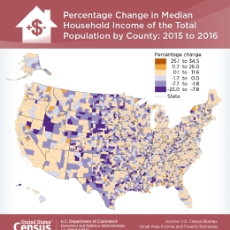
The change in median household income over the past two years for the Great Plains region can be seen in the following figure. Figure 5 displays two maps of one-year change in median household income for all counties. The top panel shows the change in median household income from 2014 to 2015, and the bottom panel shows the change from 2015 to 2016. While many of the counties in the Great Plains region saw an increase in median household income from 2014 to 2015, in the following year from 2015 to 2016, many of these same counties saw a sudden decrease in median household income. So even though median household income is still higher than it was prerecession for these counties, the growth has not been steady and has changed dramatically year-to-year.
Figure 5. Change in Median Household Income by County: 2014 to 2015 and 2015 to 2016

With SAIPE we can detect and analyze timely annual changes in income and poverty for small areas. Further analysis of state- and county-level trends of income and poverty can be found in the SAIPE report accompanying today’s release of the 2016 SAIPE program estimates. All SAIPE data can be downloaded from the SAIPE website or the Census Bureau’s application programming interface (API), giving public access to quality, single-year estimates for all counties and school districts.
Related Information

Page Last Revised - October 8, 2021
✕
Is this page helpful?
 Yes
Yes
 No
No
 Yes
Yes
 No
No✕
NO THANKS
255 characters maximum
 255 characters maximum reached
✕
Thank you for your feedback.
Comments or suggestions?

Comments or suggestions?