X-13ARIMA-SEATS Seasonal Adjustment Program
X-13ARIMA-SEATS Seasonal Adjustment Program
References
This page contains links to a number of resources for users of X-13ARIMA-SEATS, whatever their level of experience or expertise.
We will be adding to these resources over time - if you know of something that would be appropriate for this page, contact us.
Resources for New Users
Listed here are materials developed to new users understand the seasonal adjustment method contained within X-13ARIMA-SEATS.
Seasonal Adjustment FAQs and Tutorials
Listed here are more materials developed to help the user understand the seasonal adjustment method contained within X-13ARIMA-SEATS.

Seasonal Adjustment Questions and Answers
A time series is a sequence of successive measurements of values obtained at regular time intervals (such as every month or every quarter).
For most types of time series analysis, the data must be comparable over time, so they must be consistent in concept and the method of measurement. Many of the Census Bureau’s time series measure economic activity and are inputs to estimates of the GDP.
Seasonal adjustment is the estimation and removal of seasonal effects from a time series to reveal certain nonseasonal features. Seasonal effects are the persistent, repeated effects that occur at the same time each year, and that are not explainable by the dynamics of trends or cycles. Examples of seasonal effects include a July drop in automobile production as factories retool for new models, and increases in heating oil production during September in anticipation of the winter heating season.
When appropriate, the seasonal adjustment process estimates and removes not only seasonal effects but also calendar effects. These are consistent, predictable effects that are not strictly seasonal, such as trading day effects (related to months or quarters having different numbers of each day of the week from year to year, see Question 7 and moving holiday effects (for example, Labor Day, Thanksgiving, and Easter, see Question 9.
We call the numerical estimates of these effects “factors,” and the estimates of the seasonal factors along with the calendar effects “combined factors.” Commonly, although we adjust for combined effects, we use the general terms “seasonal adjustment” and “seasonal factor” to describe the adjustment. By convention, we use the word factor, which implies a multiplicative nature of the effects, even when the effects have an additive nature.
Seasonal movements are often large enough that they mask other characteristics of the data that are of interest to analysts of current trends and cycles.
For example, if each month (or quarter) has a different seasonal tendency toward high or low values, it can be difficult to detect the general direction of a time series' recent monthly (or quarterly) movement (increase, decrease, change of direction, no change, consistency with another economic indicator, etc.).
Seasonal adjustment produces a time series whose neighboring values are usually easier to compare.
Many data users prefer seasonally adjusted data to the original time series, because they want to see the characteristics that seasonal movements tend to mask, especially changes in the direction of the series.
This difference in direction is common. In the case of an increase in the original (not seasonally adjusted) series and a decrease in the seasonally adjusted series, the usual reason is that the seasonal effect for the second month (or quarter) is larger than the seasonal effect for the first month (or quarter). If the underlying level of the series were steady, the first value would be larger than the second value because of the seasonal effect. In this scenario, the original series' increase must be smaller than usual, either because the underlying level of the series is decreasing or because some special event (or events) increased the first month’s (or quarter’s) value or decreased the second month’s (or quarter’s) value. Note that if the series is adjusted for trading day or moving holiday effects, other explanations are possible.
The seasonally adjusted series can increase when the original series decreases, as well.
See the graph below of an overlay of an original (not seasonally adjusted) monthly series in gray and its corresponding seasonally adjusted series in blue. In 2017, the original series increased from January to February, and the seasonally adjusted series decreased (other months also show a difference in direction). Note that the up and down movements in a time series might not be statistically meaningful and might not warrant any particular interpretation.
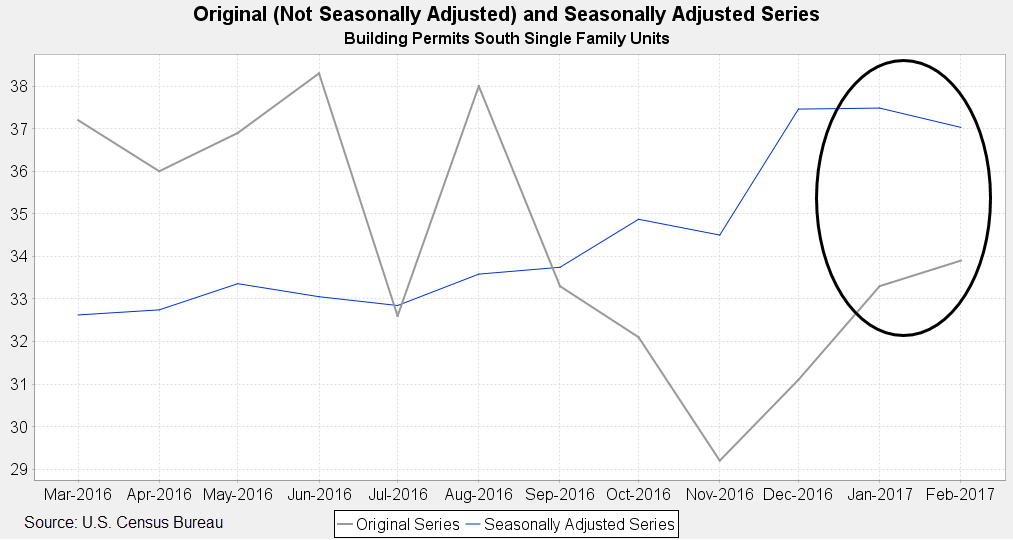
Figure 1. Original (Not seasonally Adjusted) and Seasonally Adjusted South Single Family Building Permits. Source: U.S. Census Bureau.
The goal of seasonal adjustment is to estimate the effects that occur in the same calendar month or quarter and have similar magnitude and direction from year to year. Seasonal adjustment of monthly retail sales removes an average increase in Christmas sales in December. However, an unusually high value resulting from sales of an innovative new product will still be noticeable in the seasonally adjusted series. In series whose seasonality results primarily from weather, the estimated seasonal factors are average weather effects. For example, the average decrease in new home construction in the Northeastern region in winter months due to cold and storms results in lower seasonal factors in those months. Seasonal adjustment does not account for abnormal weather conditions or for sudden changes in weather patterns. In addition, abnormal weather that occurs in one geographic location might not have any discernable effect on the U.S. total.
It is important to note that seasonal factors are estimates based on present and past experience, and that future data may show a different pattern of seasonal effects. Particularly high levels of noise or unusual events that occur at the same time in successive years can impede this estimation.
Seasonal adjustment separates a time series into trend-cycle, seasonal, and irregular components.
Trend-Cycle (C): Level estimate for each month (or quarter) derived from the surrounding year-or-two of observations. This component shows the long-term movement of the time series.
Seasonal component (S): Effects that are reasonably stable in terms of annual timing, direction, and magnitude. Possible causes include natural elements (usual weather patterns), administrative measures (starting and ending dates of the school year), and social/cultural/religious traditions (fixed holidays such as Christmas). If the series is affected by trading day or moving holiday effects, we include adjustments for these with the seasonal component, even though they are not strictly seasonal. We often publish the seasonal, trading day, and moving holiday effects as one combined factor, labeled simply as a seasonal factor.
Irregular component (I): Anything not included in the trend-cycle or the seasonal (or combined) component. Its values are unpredictable with respect to timing, impact, and duration. It can arise from sampling error, non-sampling error, unseasonable weather, natural disasters, strikes, etc.
These have a multiplicative or an additive relationship, depending on the nature of the time series. That is, the original series equals C x S x I, when the relationship is multiplicative, and it equals C + S + I, when the relationship is additive.
If the variance of the series generally increases as the level increases, the components have a multiplicative relationship. If the variance of the series remains steady regardless of the level of the series, the components have an additive relationship. This nature of the series can be difficult to determine and can change over time.
Recurring effects associated with the days of the week are trading day effects. Monthly (or quarterly) time series values might depend on the weekday composition of the calendar month (or quarter). Activity level might depend on which days of the week occur five times in the month instead of only four times, or which days of the week occur 14, 13, or 12 times within the quarter. For example, building permit offices usually are closed on Saturday and Sunday. Thus, the number of building permits issued in a given month is likely to be higher if the month contains more weekdays and lower if the month contains more weekend days.
Flow time series, those whose values accumulate over time (sales, for instance) might depend on the number of each day of the week in the month (or quarter). Stock time series, those whose values represent a snapshot in time (inventories, for instance), might depend on the day of the week when they are measured. For example, inventory values at the end of the month (or quarter) might be lower if the last day is Wednesday than if the last day is Friday, if new stock always arrives on Thursday.
Trading day effects can make it difficult to compare series values or to compare movements in one series with movements in another. When appropriate for the series, and when estimates of trading day effects are statistically significant, we remove them from the series. Trading day adjustment is the removal of such estimates. Usually we do not publish separate trading day factors, which are the estimates of these effects. Instead, we publish combined effects, which include the trading day factors implicitly. By convention, we usually label the combined effects simply as seasonal factors.
For flow time series, whose values accumulate over time, leap-year effects are part of the trading day estimation and adjustment, which is part of the seasonal adjustment process, when it is appropriate for the series and the effect is statistically significant. For a multiplicative adjustment, February estimates are rescaled by multiplying the estimate by the ratio of the average length of February (28.25 days) to the length of the given February (either 28 or 29 days). For an additive adjustment, the regression model includes a leap-year regressor.
For stock (inventory) series, we generally do not adjust for leap-year or length-of-month (or length-of-quarter) effects.
Holidays whose effects always fall in the same month (or quarter) each year are merely part of the typical seasonal pattern and seasonal adjustment process. However, holidays whose effects move between or among months (or quarters) from year to year are called moving holidays. Moving holiday adjustments are the estimation of those effects by regression and their removal from the time series.
For instance, the moving holiday with the most impact on Census Bureau series is Easter, which can fall in March or April (or in Quarter 1 or Quarter 2). When Easter is in March, we expect to see higher sales at clothing stores in March as people buy new outfits for the holiday; when Easter is in April, that increased activity may fall entirely in April or it may be split between March and April, depending on how close to the beginning of the month Easter falls.
For moving holidays like Easter (or Labor Day, Thanksgiving, or other recurring events), the regression effects reflect the proportion of the window of the holiday period that falls in each month (or quarter, if applicable). For instance, if the Easter effect is determined to occur in the eight days before Easter, and Easter falls on April 4, then 5/8 of the effect is in March and 3/8 of the effect is in April. If Easter falls on April 1 (or earlier), then the entire effect is in March. If Easter falls on April 9 (or later), then the entire effect is in April.
Labor Day is always in September and Thanksgiving is always in November, but the window of the holiday period is proportioned differently among months from year to year. For instance, if the window of the Thanksgiving holiday period is determined to start the day after Thanksgiving and continue through December 24, then if Thanksgiving falls early in November, we expect more of the Christmas shopping activity to occur in November; if Thanksgiving is late in November, we expect less of the Christmas shopping activity to occur in November.
Analysts determine the length of the holiday window based on knowledge of the time series subject matter and tests of the significance of the regression effects. For a given month, the regression variable for the holiday effect is the proportion of the affected time period that falls in that month (in the Easter example above, 5/8 in March and 3/8 in April). The regressors are centered by subtraction of their long-term means, so they are not the exact simple proportions.
When appropriate for the series, and when the effect is statistically significant, we estimate and remove it from the series. We combine the moving holiday factors with the seasonal factors and trading day factors to produce combined factors, typically published and labeled simply as the seasonal factors.
We use X-13ARIMA-SEATS software to derive our seasonal adjustment and produce seasonal factors.
Estimating seasonal effects is difficult when the underlying level of the series (the trend-cycle) changes over time. Estimating the underlying level of the series is difficult in the presence of seasonal effects. For these reasons, the X-11 seasonal adjustment method available in X-13ARIMA-SEATS uses an iterative procedure of deriving component estimates, with successive improvements. It starts by removing a crude, preliminary estimate of the trend-cycle. It then derives crude seasonal factors from the de-trended series. It removes these seasonal effects to derive a better estimate of the trend-cycle, allowing for a better estimate of the de-trended series, which leads to more refined seasonal factors. The process uses crude, and then successively more refined, irregular component estimates to identify and replace extreme values that can distort the estimates of trend-cycle and seasonal factors.
The SEATS (Signal Extraction in ARIMA Time Series) seasonal adjustment method available in X 13ARIMA-SEATS uses parameter estimates from autoregressive integrated moving average (ARIMA) models to filter the series and derive the seasonal factors and other components.
For many time series, a multiplicative seasonal adjustment is appropriate, and the seasonally adjusted series is the original series divided by the seasonal (or combined) factors. For example, suppose for January 2017, a series has an original value of 100,000 and a multiplicative seasonal factor of 0.80. The seasonally adjusted value for January 2017 is 100,000/0.80 = 125,000.
For some time series, an additive seasonal adjustment is appropriate, and the seasonally adjusted series is the original series minus the seasonal (or combined) factors. For example, suppose for January 2017, a series has an original value of 90,000 and an additive seasonal factor of -10,000. The seasonally adjusted value for January 2017 is 90,000 – (-10,000) = 100,000.
If appropriate, we fit regression effects along with the ARIMA models to estimate trading day and/or moving holiday effects, and the software removes these effects from the series before estimation of the pure seasonal, trend-cycle, and irregular components. The resulting seasonally adjusted series is therefore the result of dividing by (or subtracting) the combined trading day, holiday, and seasonal factors. Many tables refer to the combined factors as the seasonal factors for simplicity.
The seasonal adjustment procedures can produce distorted estimates of the seasonal factors if a series has an unusual value or a sudden shift in values. For that reason, we adjust series for outliers using regression effects before seasonal adjustment. These outlier effects are an important part of the economic story the series tells, however, and so they are returned to the seasonally adjusted series after the final estimation of the seasonal factors.
The models (regression combined with ARIMA, or regARIMA) also provide forecasts of series values for the estimation during the filtering, whether that is with the X-11 or SEATS method.
X-13ARIMA-SEATS is a seasonal adjustment software program developed and maintained at the U.S. Census Bureau. The program is an expansion of the Census Bureau's earlier X-12-ARIMA program, which itself was an expansion of the initial X-11 software from the Census Bureau and X-11-ARIMA from Statistics Canada under Estela Dagum.
The X-13ARIMA-SEATS software allows for the same adjustment methods as X-12-ARIMA and offers improvements in diagnostics as well as an enhanced version of the Bank of Spain's SEATS software. The SEATS routines are the result of collaboration with the developers of the software (Agustin Maravall, Former Chief Economist of the Bank of Spain, now retired, and Gianluca Caporello).
Improvements in X-13ARIMA-SEATS as compared to X-12-ARIMA include
- additional regressors for modeling calendar effects in stock (inventory) time series
- built-in regressors for new outlier types, including seasonal outliers, quadratic ramps, and temporary level shifts
- the ability to designate groups of user-defined holiday regressors and generate model diagnostics for the different groups
- regression model-based F tests for stable seasonal and trading day regressors
- accessible HTML output generated directly by the software rather than by a separate utility.
Annually, many program areas release summary measures as listed below, at least for major aggregates or high-profile individual series. Look for this kind of information in the methodology descriptions of the economic indicators.
- For multiplicative adjustments, average percentage change (or for additive adjustments, average change), with outlier effects removed, in the
- Original series
- Seasonally adjusted series, the product (or sum) of the Trend-Cycle and Irregular components
- Trend-Cycle component
- Irregular component
- Months (or quarters) for cyclical dominance
| Name | Description |
|---|---|
| Average change in the original series | For series with a multiplicative effect, the average month-to-month (or quarter-to-quarter) percentage change, without regard to sign, of the seasonally adjusted series after removal of outlier effects. For series with an additive effect, the average month-to-month (or quarter-to-quarter) change, without regard to sign, of the original (not seasonally adjusted) series after removal of outlier effects. |
| Average change in the seasonally adjusted series | For series with a multiplicative effect, the average month-to-month (or quarter-to-quarter) percentage change, without regard to sign, of the seasonally adjusted series after removal of outlier effects. For series with an additive effect, the average month-to-month (or quarter-to-quarter) change, without regard to sign, of the seasonally adjusted series after removal of outlier effects. |
| Average change in the trend-cycle component | For series with a multiplicative effect, the average month-to-month (or quarter-to-quarter) percentage change of the trend-cycle component after removal of outlier effects. For series with an additive effect, the average month-to-month (or quarter-to-quarter) change of the trend-cycle component. The trend-cycle component is a smoothed version of the seasonally adjusted series obtained by means of a moving average after removal of outlier effects. |
| Average change in the irregular component | For series with a multiplicative effect, the average month-to-month (or quarter-to-quarter) percentage change of the irregular component. The irregular component is equal to the seasonally adjusted series divided by the trend-cycle component after removal of outlier effects. For series with an additive effect, the average month-to-month (or quarter-to-quarter) change of the irregular component. The irregular component is equal to the seasonally adjusted series minus the trend-cycle component after removal of outlier effects. |
| Months (or Quarters) for Cyclical Dominance | An estimate of the appropriate time span over which to consider cyclical movement in a time series, or in other words, it is the shortest span of time for which the average change (without regard to sign) in the trend-cycle component is larger than the average change (without regard to sign) in the irregular component. It provides a measure of how long before fluctuations begin to be more attributable to cyclical than to irregular movements. Usually this measure is smaller for series with stable patterns and larger for series that are more volatile. Note however, that for series whose trend-cycle is relatively flat (not increasing or decreasing appreciably over time), this measure typically is large, regardless of the stability of the series’ patterns. |
X-13ARIMA-SEATS software produces much diagnostic information. For modeling, we use standard diagnostics, often of a comparative nature, to choose models with lower forecast error, better goodness of fit, and residuals that appear serially uncorrelated. When selecting seasonal adjustment settings, we consider a variety of diagnostics. To judge the quality of a seasonal adjustment, we primarily consider diagnostics that indicate whether the adjusted series shows signs of significant residual seasonality and how stable the adjustment is, that is, how large the revisions to the estimated seasonal factors are as we add more series values.
- No evidence of significant residual seasonality
After we have seasonally adjusted a time series, it should have no significant seasonal effects remaining (no residual seasonality). X-13ARIMA-SEATS has diagnostic tests for seasonality that we review. As with all statistics, these are subject to uncertainty. These tests include- Maravall’s QS diagnostic, a check of the autocorrelation at seasonal lags of the seasonally adjusted series. The diagnostic follows an approximate chi-squared distribution, and an associated p-value of less than 0.01 indicates possible residual seasonality.
For monthly time series, reviewers might check the result of Maravall’s QS diagnostic for the collapsed quarterly versions of the series if the monthly series are inputs to quarterly GDP estimates. - For monthly series, the spectrum of the seasonally adjusted series. A tall peak of six or more stars at any of the seasonal frequencies 1/12, 2/12, 3/12, or 4/12 indicates possible residual seasonality. It is considered as a peak only if it is taller than the median level of all of the measured frequencies. (The unit of measure is a “star” because the graphs originated in text files where the seasonal frequencies were indicated with asterisks. One star is 1/52 of the range of the heights of the measured frequencies.)
- Maravall’s QS diagnostic, a check of the autocorrelation at seasonal lags of the seasonally adjusted series. The diagnostic follows an approximate chi-squared distribution, and an associated p-value of less than 0.01 indicates possible residual seasonality.
- Stability (small revisions) of the estimates
X-13ARIMA-SEATS has stability diagnostics to help select X-13ARIMA-SEATS adjustment options that result in smaller revisions, in comparison to other sets of adjustment options. These include- Sliding spans, comparisons of seasonal adjustments of overlapping subspans of the time series. For example, how do the seasonal adjustments differ when estimated over the four subspans 2006-2016, 2007-2017, 2008-2018, and 2009-2019 from within the full time series?
- Revisions history, comparisons of lagged seasonal adjustments, usually comparisons of the initial estimates when that time point is the last value of the series (sometimes called the concurrent estimate) to the estimates for those same time points when the full time series has more data.
We revise the seasonal adjustment (and the seasonal factors) for two main reasons.
- We revise the seasonally adjusted series when we revise the original series, in order to achieve a better fit to the revised data.
- We revise some past factors as new series values become available. We use the new values to improve the estimated seasonal adjustments of the most recent years. For instance, the estimate of a seasonal factor for January 2015 is most strongly influenced by the estimates of surrounding Januaries (especially from 2014 and 2016). In 2015, before January 2016 and later values were available, the seasonal factor estimate for January 2015 was less reliable. We will revise the estimate of the January 2015 seasonal factor to incorporate the information from the new series values.
Very generally, what we call the seasonally adjusted annual rate for an individual month (or quarter) is an estimate of what the annual total would be if non-seasonal conditions were the same throughout the year. This "rate" is not a rate in a technical sense, but is rather a level estimate.
For a monthly series, the seasonally adjusted annual rate is the seasonally adjusted value multiplied by 12; for a quarterly series, it’s multiplied by 4.
The annual rate allows us easily to compare one month's value or one quarter's value to an annual total, and to compare a month to a quarter.
The Bureau of Economic Analysis (BEA) publishes quarterly estimates of the U.S. GDP at an annual rate, and many of the Census Bureau data series are inputs to GDP. Annual rates for the input series help users see the data at the same level as GDP estimates.
When multiplicative seasonal adjustment is derived by dividing the time series by seasonal factors (or combined factors), it is arithmetically impossible for the adjusted series to have the same annual totals as the original series. Even with additive seasonal adjustment, this relationship is possible only in the uninteresting case in which the seasonal pattern repeats perfectly from year to year and the series has no trading day (or leap year) effects. Even in that case, even simple rounding of the seasonal factors could produce an inequality. "Benchmarking" methods can force the adjusted series to have the same totals as the original series, but these procedures do not account for evolving seasonal effects or for trading day differences due to the differing weekday compositions of different years. X-13ARIMA-SEATS has methods to keep the annual sums close to the sum of the individual component months or quarters while still allowing for changes over time and the trading day effects.
For monthly flow series, such as sales, summing the monthly seasonally adjusted values or averaging the monthly seasonally adjusted annual rate values over a quarter produces a corresponding seasonally adjusted value for the quarter.
For monthly stock (inventory) series, we usually take the seasonally adjusted value for the last month of the quarter as the corresponding seasonally adjusted value for the quarter.
Note that these methods will not produce the same result as directly seasonally adjusting the quarterly series.
Concurrent adjustment is the adjustment resulting from using all available time series values up to and including the current month (or quarter). In the earliest days of seasonal adjustment, the available computing power made concurrent seasonal adjustment all but impossible, so most seasonal adjustment used projected factors computed once a year. Some program areas still use projected factors so that they know what the seasonal factors will be for the upcoming year. Projections might occur more than once a year, such as once a quarter or with other timing.
Because concurrent seasonal adjustment uses more of the available information for each adjustment, it is usually closer to the final seasonal adjustment than the projected adjustment is, especially as the length of time increases from when the projections occurred.
Some sources use the expression concurrent adjustment to refer only to the adjustment of the most recent value of the time series, leaving it unclear as to how to refer to the time points prior to the latest. We tend to use the expression more generally, to refer to the adjustment of the entire series including that latest and newest value and potentially revised estimates of previous values.
An indirect adjustment is a composite of other seasonal adjustments. It can take various forms.
For instance, if a time series is a sum of seasonal component series, then the sum of each seasonally adjusted component provides an indirect seasonal adjustment of the aggregate. This adjustment can differ greatly from the direct seasonal adjustment of the aggregate original (not seasonally adjusted) series.
For example,
United States = Northeast Region + Midwest Region + South Region + West Region
Indirect SAdj (U.S.) = SAdj (NE) +
SAdj (MW) + SAdj (S) + SAdj (W)
Direct SAdj (U.S.) = SAdj (NE + MW + S +W)
where “SAdj (series)” indicates the seasonal adjustment of the series.
Because seasonal patterns differ by region, we adjust at the regional level and sum the results to obtain the seasonal adjustment for the U.S. total, preserving the nature of the aggregation.
Note that indirect adjustment is not limited to additive relationships. For example, to derive the seasonally adjusted trade balance, add the seasonally adjusted export values and subtract the seasonally adjusted import values. Other forms of indirect adjustment are also possible.
When the component series have distinct seasonal patterns and have adjustments of good quality, we often prefer an indirect seasonal adjustment. Some data users prefer indirect seasonal adjustments because they maintain a consistent relationship between the component series and the aggregate.
X-13ARIMA-SEATS provides diagnostics for direct and indirect seasonal adjustments to help reviewers choose adjustment settings.
Guidelines for Seasonal Adjustment
These documents contain guidelines for using seasonal adjustment diagnostics available from X-13ARIMA-SEATS and other seasonal adjustment packages from the Census Bureau and other statistical agencies.

Documentation for X-13ARIMA-SEATS and related programs
Documentation, quick references, and other material useful to those who run X-13ARIMA-SEATS are given below: