The BDS-HG experimental data product classifies firms by their growth rate between t-1 and t as described in Kim et al. (2024). Here we briefly summarize the methodology describe by Kim et al. (2024). Firm-level growth rates are computed as the aggregation of establishment-level changes in employment divided by the sum of average establishment between t-1 and t. Specifically, establishment growth g_it is defined as follows:

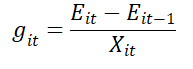
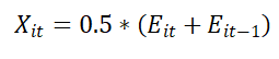
For establishment i at time t with employment E. The denominator, X_it is defined as follows:

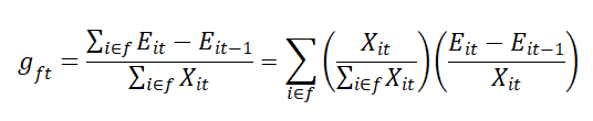
Firm-level growth, g_ft, is then the sum of employment changes weighted by the sum of average establishment employment, for all establishments i associated with firm f at time t. This is computed as follows:

This growth rate measure, first developed by Tornqvist et al. (1985), has become standard in the firm dynamics literature (Davis et al., 1996). g_ft is bounded from -2 to 2 with firms that transition from positive to zero employment having a firm growth rate of -2 and firms that transition from zero employment to positive employment having a growth rate of 2.

This growth measure has a number of desirable properties. First, it approximates log differences when growth rates are near zero. Second, it can be easily aggregated across cells given information about positive and negative changes and the sum of average employment. Third, it is defined for both entrants and exits. Fourth, it is symmetric for employment increases and decreases. For example, an establishment that changes from 10 to 15 employees will have a g_it growth rate of 0.4 (50% increase) and an establishment that changes from 15 to 10 employees will have a growth rate g_it of -0.4 (-33% decrease).

There are two firm-level growth rate classifications used in the BDS-HG tabulations. The first classifies firms by their firm growth rate g_ft in a given year (fempgr_gr). This classification uses the following nine bins: a) -2; b) (-2 to -0.8]; c) (-0.8 to -0.2]; d) (-0.2 to -0.01]; e) (-0.01 to 0.01); f) [0.01 to 0.2); g) [0.2 to 0.8); h) [0.8 to 2); i) 2. Note that the bins area not of equal size. Firms that enter (2) or exit (-2) are classified separately. Moreover, firms with growth rates near but not exactly zero are grouped together ((-0.01 to 0.01)).

The second firm growth classification identifies where a given firm sits on the within-year average employment weighted firm growth rate distribution (fempgr_grpct). To compute weighted percentiles, we order firms within a given year by their firm growth rates g_ft, breaking ties randomly, and compute the cumulative share of total average employment. The cumulative share of total average employment is then used to assign firms to one of five percentile-based bins as follows: a) [0 to 10], b) (10 to 25], c) (25 to 75], d) (75 to 90], e) (90 to 100]. Again, bins are not equally sized. This method, by construction, involves cut-offs that vary over time. As the firm growth rate distribution changes over time so too will the percentile-based cutoffs. This is illustrated in Figure 1 of Kim et al, shown below. The growth rate associated with the employment-weighted 90^th percentile fell from 0.35 in the late 1970s to 0.23 in the 2010s.

Figure 1: Firm growth rates by percentile over time

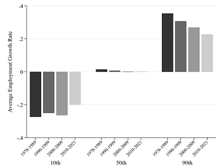
Source: Kim et al. (2024), Figure 1.

For more information about the BDS-HG methodology and firm growth rates in the LBD see Kim et al. (2024).

References

i. Kim, J.D., Choi, J., Goldschlag, N., Haltiwanger, J. (2024). High-Growth Firms in the United States: Key Trends and New Data Opportunities. CES Discussion Paper Series, CES-WP-24-11, Center for Economic Studies, U.S. Census Bureau.

ii. Davis, Steven J, John Haltiwanger, and Scott Schuh (1996) Job Creation and Destruction: MIT press.

iii. Törnqvist, Leo, Pentti Vartia, and Yrjö O Vartia (1985) “How should relative changes be measured?” The American Statistician, 39 (1), 43–46.